Traditional real-time object detectors like YOLO do a great job balancing speed and accuracy, but they often struggle with pinpointing exact object locations because they rely on fixed-coordinate bounding boxes.D-FINE takes a fresh approach by treating bounding box regression as a fine-grained distribution refinement process. [1]
This means instead of just predicting static coordinates, it refines object locations step by step, leading to more precise detections without sacrificing speed. The result? D-FINE outperforms many existing models in real-time settings, making it a solid choice for resource-limited environments like mobile devices and edge computing.
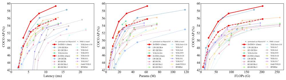
Comparisons with other detectors in terms of latency (left),model size (mid), and computational cost (right). We measure end-to-end latencyusing TensorRT FP16 on an NVIDIA T4 GPU. [2]
Challenges in Traditional Object Detection
Object detection algorithms typically use one of two main approaches:
Anchor-based detectors (e.g., Faster R-CNN) that rely on predefined anchor boxes.
Anchor-free detectors (e.g., DETR) that directly predict object locations and categories.
While DETR (Detection Transformer) models eliminate the need for anchors and non-maximum suppression (NMS), they suffer from high computational costs and suboptimal bounding box regression. D-FINE addresses these issues through:
Fine-grained Distribution Refinement (FDR): Transforming bounding box regression into an iterative probability distribution refinement process.
Global Optimal Localization Self-Distillation (GO-LSD): Enhancing localization precision by transferring knowledge from refined distributions to earlier layers.
What is D-FINE?
D-FINE builds upon the DETR framework and introduces two core innovations: FDR and GO-LSD, which redefine bounding box regression and optimize knowledge transfer.
How D-FINE works?
1. Fine-Grained Distribution Refinement (FDR)
Traditional bounding box regression methods predict fixed coordinates, often leading to imprecise localization. Instead of predicting absolute coordinates, FDR models bounding boxes as probability distributions that are iteratively refined.
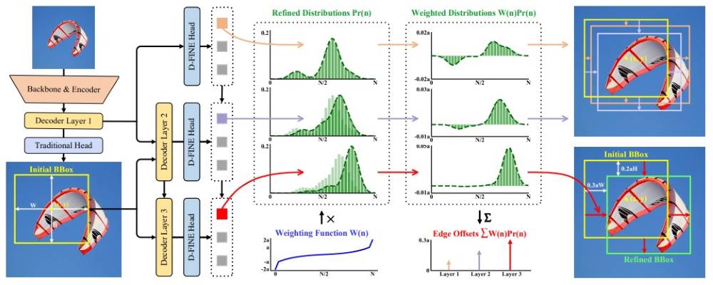
Overview of D-FINE with FDR. The probability distributionsthat act as a more finegrained intermediate representation are iterativelyrefined by the decoder layers in a residual manner. Non-uniform weightingfunctions are applied to allow for finer localization. [2]
How FDR Works:
Each bounding box is represented by four probability distributions (one for each edge: top, bottom, left, and right).
The model iteratively refines these distributions across decoder layers, progressively improving localization accuracy.
A non-uniform weighting function is applied to the distributions, allowing finer adjustments near the true bounding box location.
By adopting this approach, FDR enables progressive fine-tuning of object boundaries, leading to superior localization precision.
2. Global Optimal Localization Self-Distillation (GO-LSD)
To further enhance localization accuracy, GO-LSD distills refined bounding box knowledge from deeper layers to shallower ones. This bidirectional optimization technique enables:
Early-stage layers to produce better initial bounding box predictions.
Later-stage layers to focus on smaller residual refinements.
Faster model convergence by improving gradient flow.
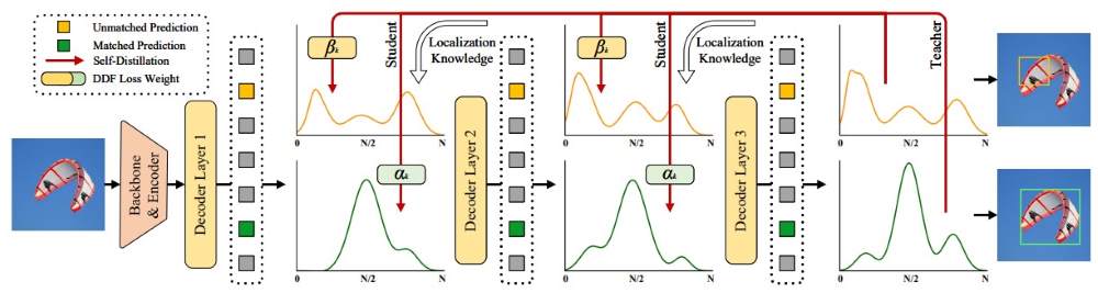
Overview of GO-LSD process. Localization knowledge from the final layer’s refined distributions is distilled into shallower layers through DDF loss with decoupled weighting strategies. [2]
Key Features of GO-LSD:
Hungarian Matching: Ensures precise one-to-one matching of predictions and ground truth objects across layers.
Decoupled Distillation Focal (DDF) Loss: A novel loss function that prioritizes well-localized but low-confidence predictions, ensuring optimal knowledge transfer.
By aligning the predictions of early decoder layers with the refined distributions of later layers, GO-LSD accelerates training and improves overall detection accuracy.
Performance Evaluation
D-FINE is benchmarked on the COCO dataset, comparing against state-of-the-art real-time detectors like YOLOv10 and RT-DETR.
Key Results:
D-FINE-X achieves 55.8% AP (Average Precision) at 78 FPS on an NVIDIA T4 GPU, outperforming competitors.
Pretraining on Objects365 boosts D-FINE-X to 59.3% AP, surpassing all existing real-time detectors.
Improves existing DETR models by up to 5.3% AP with negligible additional training cost.
Advantages of D-FINE
Open-Source Licensing: 🎉
- YOLOv8 and YOLO11 are powerful, but their AGPL-3.0 licenses can be a dealbreaker—especially for SaaS, where you might have to open-source your whole project.
- D-FINE, on the other hand, comes with the Apache 2.0 license, meaning you can use, modify, and sell it without the legal drama. More freedom, no headaches.
Higher Localization Accuracy: The fine-grained distribution approach significantly reduces bounding box errors.
🚀 Faster Convergence: GO-LSD enables efficient self-distillation, improving model training efficiency.
Real-Time Performance: Optimized transformer modules ensure low latency while maintaining high detection precision.
Lightweight Design: D-FINE maintains a smaller computational footprint compared to traditional DETR models.
Conclusion
D-FINE revolutionizes object detection by redefining bounding box regression as a probability distribution refinement task. With FDR and GO-LSD, the model achieves state-of-the-art localization accuracy while maintaining real-time performance.Future work will focus on enhancing lightweight variants of D-FINE for mobile and edge AI applications, ensuring that high-precision object detection is accessible across a wide range of devices.
The Ikomia API allows to train and infer D-FINE object detector with minimal coding.
Setup
To begin, it's important to first install the API in a virtual environment [3]. This setup ensures a smooth and efficient start to using the API's capabilities.
The Ikomia API allows to train and infer D-FINE object detector with minimal coding.
pip install ikomia
Dataset
For this tutorial, we're using a License plate dataset [4] from Roboflow with 200images to illustrate the training of our custom D-FINE object detection model.
Train D-FINE with a few lines of code
You can also directly charge the notebook we have prepared.
from ikomia.dataprocess.workflow import Workflow
import os

#----------------------------- Step 1 -----------------------------------#
# Create a workflow which will take your dataset as input and
# train a D-FINE model on it
#------------------------------------------------------------------------#
wf = Workflow()

#----------------------------- Step 2 -----------------------------------#
# First you need to convert the COCO format to IKOMIA format.
# Add an Ikomia dataset converter to your workflow.
#------------------------------------------------------------------------#

dataset = wf.add_task(name="dataset_coco")

dataset.set_parameters({
    "json_file": "path/to/_annotations.coco.json",
    "image_folder": "path/to/image/folder/train",
    "task":"detection",
})

#----------------------------- Step 3 -----------------------------------#
# Then, you want to train a D-FINE model.
# Add D-FINEtraining algorithm to your workflow
#------------------------------------------------------------------------#
train = wf.add_task(name="train_d_fine", auto_connect=True)

train.set_parameters({
    "model_name": "dfine_m",
    "epochs": "100",
    "batch_size": "8",
    "input_size": "640",
    "dataset_split_ratio": "0.8",
    "workers": "4",  # recommended to set to 0 if you are using Windows
    "weight_decay": "0.000125",
    "lr": "0.00055",
    "output_folder": os.getcwd(),
})


#----------------------------- Step 4 -----------------------------------#
# Execute your workflow.
# It automatically runs all your tasks sequentially.
#------------------------------------------------------------------------#
wf.run()
Here are the configurable parameters and their respective descriptions:
model_name (str) - default 'dfine_m': Name of the D-FINE pre-trained model on Objects365 (Best generalization). Other model available:
dfine_s
dfine_l
dfine_x
batch_size (int) - default '8': Number of samples processed before the model is updated.
epochs (int) - default '50': Number of complete passes through the training dataset.
dataset_split_ratio (float) – default '0.9': Divide the dataset into train and evaluation sets ]0, 1[.
input_size (int) - default '640': Size of the input image.
workers (int) - default '0': Number of worker threads for data loading (per RANK if DDP).
lr (float) - default '0.00025': Initial learning rate. Adjusting this value is crucial for the optimization process, influencing how rapidly model weights are updated.
output_folder (str, optional): path to where the model will be saved.
config_file (str, optional): path to the training config file .yaml. Using a config file allows you to set all the train settings available.
The training process for 100 epochs was completed in approximately 25 minutes using an NVIDIA L4 24GB GPU.
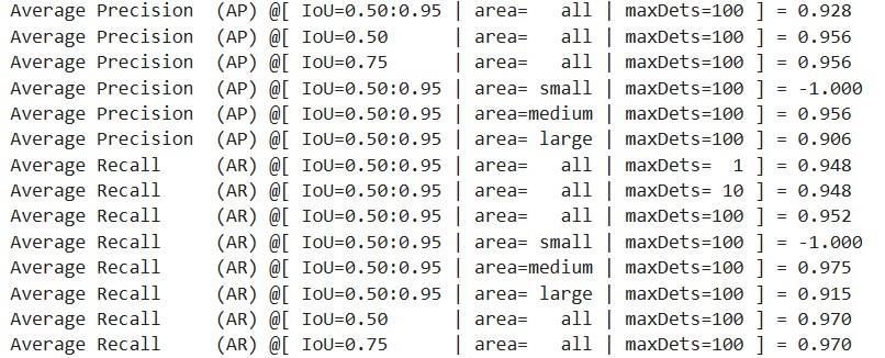
Performance of our custom D-FINE model
The best-performing model was achieved at epoch 62, with an mAP50-95 score of 0.9279. All metrics were tracked using MLflow for comprehensive monitoring and analysis.
The visualizations provide key insights into various performance metrics essential for evaluating the effectiveness of our object detection model. Observing the training and validation loss curves, both show a steady decline before reaching a plateau, indicating that the model has successfully converged without significant overfitting.
Overall, the model has learned effectively, showing high precision, recall, and mAP values.
Run your fine-tuned D-FINE model
We can test our custom model using the ‘infer_yolo_v10’ algorithm. While by default the algorithm uses the COCO pre-trained dfine_m model, we can apply our fine-tuned model by specifying the 'model_weight_file', 'config_file' and 'class_file' parameters:
from ikomia.dataprocess.workflow import Workflow
from ikomia.utils.displayIO import display

# Create your workflow for D-FINE inference
wf = Workflow()

# Add D-FINEinstance segmentation to your workflow
d_fine = wf.add_task(name="infer_d_fine", auto_connect=True)
d_fine.set_parameters({
    "model_weight_file": 'path/to/best_stg1.pth',
    "config_file": 'path/to/config_file.yaml',
    "class_file": 'path/to/class_names.txt',
    "conf_thres": "0.5",
    "input_size":"640"
})

# Apply D-FINE object detection on your image
wf.run_on(path='path/to/test/1k9uinoun9ha1_jpg.rf.ddaa941b04990f4a189d077ddbed134f.jpg'))

# Get D-FINE image result
img_bbox = d_fine.get_image_with_graphics()

# Display
display(img_bbox)
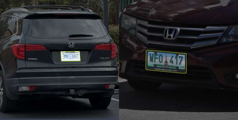
Our model successfully identified the license plate.
Chain your custom model with an OCR algorithm
One of the key strengths of the Ikomia API is its ability to seamlessly chain algorithms without worrying about input/output formats or dependency installation, even when using models from different frameworks (e.g., Hugging Face, OpenMMLab, Ultralytics).
In this example, we will perform text recognition on the bounding boxes generated by our custom model using Florence-2 OCR.
# Init your workflow
wf = Workflow()

# Add D-FINEinstance segmentation to your workflow
d_fine = wf.add_task(name="infer_d_fine", auto_connect=True)

d_fine.set_parameters({
    "model_weight_file": os.getcwd()+ f'/{TIMESTAMP}/best_stg1.pth',
    "config_file": os.getcwd()+ f'/{TIMESTAMP}/config_{TIMESTAMP}.yaml',
    "class_file": os.getcwd()+ f'/{TIMESTAMP}/class_names.txt',
    "conf_thres": "0.5",
    "input_size":"640"
})

# Add text recognition algorithm
text_rec = wf.add_task(name="infer_florence_2_ocr", auto_connect=True)

# Run the workflow on image
wf.run_on(path=os.getcwd()+"/test/1k9uinoun9ha1_jpg.rf.ddaa941b04990f4a189d077ddbed134f.jpg")

# Display results
img_output = text_rec.get_output(0)
recognition_output = text_rec.get_output(1)
display(img_output.get_image_with_mask_and_graphics(recognition_output))
Conclusion
D-FINE redefines object detection by transforming bounding box regression into a fine-grained distribution refinement process. By integrating Fine-Grained Distribution Refinement (FDR) and Global Optimal Localization Self-Distillation (GO-LSD), it achieves superior localization accuracy while maintaining real-time performance.
Our training results demonstrate high precision, recall, and mAP scores, confirming the effectiveness of the approach. Additionally, D-FINE's compatibility with Ikomia API allows seamless integration with other algorithms, such as OCR, for extended functionalities.
Build your own Computer Vision workflow
Consult the documentation for detailed API information.
Access the latest State-of-the-art algorithms via Ikomia HUB.
Use Ikomia STUDIO for an intuitive experience with these technologies.


.svg)


